Playing with Python

I didn't think it's already 2.5 years ago since I wrote my blog about creating onions (concrete section capacity graphs), until I started writing these lines now. Wow, time flies...

The funny thing is, I haven't used that MathCAD sheet that often. It had some weird behaviour in some cases, where the plot wasn't continuous. That looked horrible. And it turned out to not be as practical as I hoped, since searching for strains using given N and M combinations turned out to be quite processing heavy.

However, I was looking into Python more and more the last years. I had used it some when doing earthquake engineering around 4 years ago or so, since the FEM package Diana FEA we used at HaskoningDHV started using it as input language with the release of version 10 back then. But lately Python has gotten a lot of attention, so I started to investigate it again some more about a year ago I think?

Python notebooks

That's when I learned of JupyterLab, a browser based Python programming environment in which you can create so-called "notebook": snippets of code you can write, rearrange, supplement with markdown, etc.

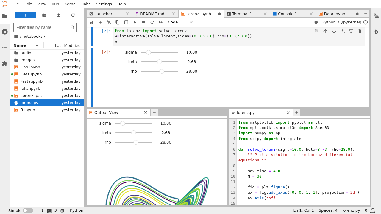
Example screenshot from the Jupyterlab website

It's versatility really surprised me to be honest! I am even starting to use MathCAD (paid software) less and less, in favor of Jupyterlab for my day-to-day calculations, although I still have to pay more attention to making my calculations better readable ;-) But it's got all the power of mathematics that MathCAD has (in libraries/packages like NumPy, SciPy, etc.) combined with the versatility of a programming language to make more powerful tools. I also think it's faster in compute-heavy calculations, but I haven't tested that yet.

Getting started

I first started with creating some basic sheets, just to get the gist of it: a simply supported beam, torsional buckling of an I-shaped beam, that sort of things. Then I started to replicate my MathCAD sheet for calculating the critical steel temperature for columns. I will not go into the code too much, you can check it here, but the result is quite nice, and very versatile!

(And for code sharing, you can use Github's Gist! See link above)

Onions again

Back to the onions. The last couple of months I have been working for a Stufib study group focusing on plasticity of concrete sections. For this, I was looking to automatically calculate the bending moment vs. the section curvature (M-Kappa diagram) for a section at different load levels. These combinations of axial load (N) and bending moment (M) are not on the M-N capacity curve of the "onion", but inside. And like I said, that had turned out kind of difficult in MathCAD. So I tried Python...

The basics for the tool/sheet/code are similar to the one in MathCAD, so for an explanation please see my blog on the MathCAD version of the onion. 

I created some functions for the onion

And beautiful onions are the result:

Next step was creating functions again, this time for drawing a M-Kappa curve at a given axial load:

Nice to know: solving capability is supported already in Python (via the SciPy package), so no writing our own Newton-Raphson iterations required. Yeah!

Then it's programming a pretty graph in Python, et voilà:

M-Kappa curves on steroids

This is nothing new, lots of software in the market already who do this flawlessly (and mind you, mine is not completely flawless yet, but a good enough proof of concept). But here comes the good stuff: after this all you need is some looping magic and you can take these calculations to a whole new level. You just have to...

... create  a range of axial loads to calculate ...

... determine the plastic and elastic bending moments at the given axial loads ...

... and calculate a range of increasing bending moments with their respective curvatures, using some Python solving qualities...

... and you will end up with another nice graph! One that those fancy commercial software packages cannot produce!

And last but not least, to check the maximum curvature with increased axial loading:

Conclusions

After playing with it for a while now, I've written some of my findings of using Python in Jupyterlab vs. MathCAD down below as a small comparisson.

Python/Jupyterlab Pros:

• Very powerful
• Fully customizable graphs
• Markdown (HTML & LaTeX style formatting of text, in both cells and graphs)
• Free!

MathCAD Pros:

• Easy-to-write
• Easy-to-read AND check (the math written is the math calculated)
• No programming experience required

That's it for this blog! The full code for both the (M)N-Kappa calculations can be found here on Github, for those interested in taking a closer look at the (proof-of-concept!) Jupyterlab Notebook code.

If you have any questions, or comments (the code is far from perfect!), please let me know!

Bulk calculation, Newton-Raphson iteration and fire resistance

Introduction to fire resistance

About a year ago my colleagues and I faced somewhat of a challenge on one of our projects: the contractor asked us to determine the critical steel temperature in case of fire for all columns througout the building we were designing at the time.

Source: https://research.bauforumstahl.de/fileadmin/user_upload/LOCAFIplus_Design_Guide_UK.pdf

There's software to do this. One profile at a time. That's quite time consuming as you can understand. So we were looking for a different approach to this problem. And yes, again for me the solution was MathCAD, this time with a slice of Newton-Raphson iteration and a sprinkle of bulk calculation.

Critical steel temperature

Determining the critical steel temperature at a given axial load is an iterative procedure. With an increase of the steel temperature, the steel strength and stiffness start to degrade. This degradation is described with (empirical?) formulas by Eurocode (NEN-)EN 1993-1-2, so at a given temperature, you can determine the residual capacity, using reduction factors on the material properties of steel (not going into too much detail, lots to write about!):

The graphs look jagged, because the code gives a number of values at a number of temperatures. In between, you are allowed to interpolate. Fortunately, MathCAD has the capacity to make an interpolated function, which we can then use to iterate towards our solution: the critical steel temperature at a given load in case of fire, by defining all relevant formulas as functions related to the temperature:

Then we use the MathCAD solve block to determine the critical steel temperature, by intersecting the (constant) function of the given load with the (linearly interpolated function) of the capacity at a given steel temperature:

Unfortunately, (I think?) we cannot use a solve block inside a MathCAD function, which we need to run this iteration on a large list of column data. So we need to implement our own solve function

Newton-Raphson saywhat?

There's all kinds of iteration functions in math. The one that I implemented here, is a Newton-Raphson iteration. I'm no mathematician, or programmer, so here's an attempt at describing what this does in normal-folk-language:

• You define a function which calculates the difference between the capacity and the given load at a random temperature
• You determine the derivative of this difference function
• You use the ratio between these two function to "travel" along the capacity curve, until you've reached the intersection between both functions, using a loop function

My first attempt at this Newton-Raphson iteration looked like this:

The  matrix collects the calculated temperature per step, the difference between capacity and given load and the derivative of this difference. The division of the last two gives the convergence, which can be compared with the given tolerance value. A larger tolerance will result in a quicker calculation, but also a larger inaccuracy of the iteration.

Now all we have to do, after inputting a large Excel sheet with all column data (section properties, buckling lengths, axial loading in case of fire, etc.), is putting this Newton-Raphson iteration to work in a bunch of functions:

Crunch a matrix with column profiles and their respective loads and geometries

Newton-Raphson-as-a-function

Et voilá, a matrix with the critical steel temperatures for all the columns in the input Excel file:

Finally, using the Excel output object in MathCAD, combining the column input sheet and the critical steel temperature output matrix, a nice overview of the relevant data can be generated:

That's it! A tool in MathCAD to automatically perform iterative calculations on large lists of structural data!

Complex Cantilevers made easy

Introduction

The last few decades, a sound structural design has more and more become a delicate balance of engineering possibilities and wishes of architect and client on one side, and safety considerations and engineering judgment on the other. Architectural designs become more and more complex, and because of the capabilities of modern day engineering tools (e.g. FEM software), structural engineers are expected to deliver on those designs. But how do you verify the results from those complex calculations?

Burj Khalifa as one of the most well-known examples of advancements in engineering
Source photo: klook.com

I always try to break complex FEM models down to existing - in Dutch so-called - "vergeet-me-nietjes" (which roughly translates in English to "forget-me-nots"). These however can become too conservative to do a good verification of the results of complex FEM models...

This got me wondering: not only FEM software evolves, but math software evolves as well. So why not try and take those "vergeet-me-nietjes" to the next level, to actually use what I was taught in university all those years ago, to advance my verification calculations as well?

So I started with a very basic example of a stability calculation: second order bending of a slender building as a result of wind loading, combined with the vertical loads in the building over the height, where some or more parameters are not constant over the height.

Point loads and moment functions

With a building tall and slender enough, a structural engineer has to take into account (amongst others) the following aspects in his design:

• determining the basic forces in the structure, both horizontal and vertical, over the height
• determining the horizontal displacements of the structure, again over the height, and
• the influence of these displacements on the primary forces in the structure

The last bullet deals with so-called second-order effects of the structure. I will go into that subject in the second part of this blog.

Calculation through "vergeet-me-nietjes" has plenty of examples on the steps above, but always depending on limited set of variables, like constant stiffness over the length/height, and/or just one or two loads. But what if the vertical load is not constant over the height of the building? Or the horizontal load? Or even the stiffness?

In a previous blog, "MathCAD in Structural Engineering" I showed how math software can be used to calculate section forces due to a variable load over the height of the building (in that case wind), using the method of integration, where

• the shear force is the first integral of the (line) load over the height and
• the bending moment is the first integral of the shear load

For a structure loaded by point loads over the height, the shear force is the sum of the point loads over the height, but how to integrate that to bending moments? Also, integration is quite heavy on the processing power of the computer. A more efficient way to calculate the bending moment over the height would be to calculate for each individual point, and then sum the results of all seperate moment lines.

The bending moment as a result of a single point load is easily calculated :

$M_{F} = F_{i} \cdot x$

For a cantilever, the bending moment along the length can then be described as:

$M_{Ed,F} = F_{i} \cdot (l_{i}-x)$

Next, using math software and vector operations, it's just a matter of a sum of the bending moments for each point load over the height, which results in a function for the total bending moment over the height:

Below two examples of a cantilever structure with a length of 80 meters, with 4 point loads on different heights:
Next up: calculating the deformations due to the point loads in above example.

Advancing simple integration schemes

Let's start with examples of aforementioned "vergeet-me-nietjes", relevant for the stability of buildings: either a point load or a bending moment at the end of a cantilever.

With both examples, it's possible to calculate the deformation along the length of the cantilever, but only the rotation of the cantilever at the end. So I got to thinking, what if there's mutiple point loads on the cantilever, how do I determine the deformation and rotation of the cantilever along the length then?

Then I very vaguely remembered two things I was taught ages ago: 

• Rotation and deformation are in one way or the other the result of integration of the bending moment
• Integration is "math" for "chopping a function into pieces and determining the area below the function".

If you look at the examples above, several integrals can be recognized: for the deformation, the variable "L" is always of an order higher than for the rotation. So the deformation is the integral of the rotation. Also, looking at the second example where the bending moment is constant over the height, we can determine that the rotation is the first integral of the bending moment. In "math":

$\varphi (x) = constant \cdot \int_{0}^{x} Mdx$
$f(x) = constant \cdot \int_{0}^{x} \varphi (x)dx$
$f(x) = constant \cdot \int_{0}^{x} \int_{0}^{x} M(x)dxdx$

where "constant" in this case equals the reciprocal bending stiffness (1/EI), to account for the (reverse) relation to the stifness of the cantilever. Which  happens to be exactly what I learned in university (but never again used since, at least not me, until now! :-) )

If you look closely at the first "vergeet-me-nietje", you can imagine it can be broken down to multiple elements of the second one:

Thus we get an integral which can handle any kind of moment function we throw at it, resulting in the rotation at any given point of the beam; if we integrate the moment function, found in the first part of this blog, twice over the length of the cantilever, we get the displacements of a cantilever loaded by random (point) loads:

The bending moment as a result of a single point load is easily calculated :

$f(z) = \frac{1}{EI} \cdot \int_{0}^{z} \int_{0}^{z} M_{tot}dzdz$

Calculation of both earlier examples of a cantilever with 4 point loads:

Fun thing is: not only the bending moment can be defined depending on z, this can be done for the stiffness (either Young's modulus E or moment of inertia I). Just keep in mind, that the stiffness parameter depending on z then needs to be included inside the integration!

Below two variations of the first example above: in the first variation, the bottom half of the cantilever is 4 times stiffer than the top half, in the second one these stiffnesses are switched:

Now it's possible to more accurately calculate bending moments and deflection of tall, slender buildings like the Burj Khalifa at the start of this blog, with a calculation sheet no longer than page :-)

In my next blog, introducing a rotation spring at the foundation and calculating second order effects on the whole cantilever with horizontal and vertical loads alike...

* FYI, all results have been verified using FEM beam calculations *

* Just make sure shear deformation is eliminated in the verification calculations *

Onions

I am a long-time fan of onions. Raw, baked, in my salad or on my burger! But ... also onions in structural engineering, a.k.a. the concrete M-N-capacity curves for reinforced concrete sections:

My first introduction with the Onion was the in the Concrete Section Analysis (CSA) module of ESA Prima Win, the predecessor of the FEM software package SCIA Engineer. Of course there were and are more similar tools, but what has always been lacking in my opinion, was a way to do a "quick and dirty" design check on multiple combinations of normal forces (N) and bending moments (M).

Up until a few months ago, I myself mostly used tools like Technosoft's (Dutch-only software) "Kolomwapening" (Concrete column reinforcement) or "MN-Kappa" (for general concrete sections), or previously mentioned ESA (until ESA Prima WIN stopped to exist and the functionality of CSA ceased to exist). I even used IDEA's Statica once or twice the last few years.

The problem with those tools is that they are designed to (extensively) check sections: large numbers of options and settings in the software and not always the possibility to check a number of section force combinations at once.

So I first started to develop an easy Excel sheet to create a concrete "onion", based on some work of a colleague of mine at my previous employer (still a big fan, Sander!) His sheet of course was way too difficult for me, with complex VBA scripting, self-programmed Newton-Raphson iterations, crack width calculation, prestressing, etc. But it was a good starting point for my next exercise: how to create

The Onion

The basis in Excel was quite rudimentary: a fixed set of calculation lines, with varying strains on each line following the graph outline, calculating internal section forces and eventually the external section forces.

The general idea is to vary the strains in the section as follows:

(0) Full (plastic) pressure
(1) To full (plastic) tension in rebar side 1
(2) To full (plastic) tension in  rebar side 2
(3) To full (plastic) pressure in concrete outer fiber side 1
(4) To full (plastic) pressure in concrete outer fiber side 2

This is quite easy in Excel for one type of section (rectangular). The sheet below is the "background" calculation sheet:

Just add a presentable front sheet, with input options, capacity graph and the possibility to plot sets of M-N data, and you've got yourself a nice design sheet for ultimate limit capacities.

The result is also very robust (no VBA programming!), but unfortunately very limited in use (only rectangular sections, the accuracy of the graph is limited/fixed, etc.)

So I started to think on moving to MathCAD. There were 2 major steps to consider first:

1. How to (automatically) calculate internal and external forces
2. How to incorporate the strain flow described above and combine it with the calculations of internal forces

The first step 

screamed "FUNCTIONS!", see also my previous blog post about pile groups. So I started to define calculation of steel and concrete stresses based on strains, to internal forces, to external section forces. I've shown the used functions below, for those who are interested:

The result is fun, and can be easily visualized by plotting the functions, e.g. stresses and strains over the height of the section, with the corresponding external section forces:

The second step

was a bit harder. How to plot a graph in MathCAD with M-N relation, where N is not a function of M, or vice versa? So I tried a "step-wise" graph: Just define steps 0 to for strain (a function with 4 sections, one for each trajectory on the onion contour), make the strain follow the onion contour step by step, calculate M and N for these steps and plot those in relation to the steps counter. Somehow this worked almost immediately with function generated strains:

But... why not existing software?

First off, input is easy! The functions for generating the graph, can be hidden. That way, input and graph will fit on one A4:

Next: the way the calculation has been poured into functions, makes it usable in MathCAD Solve blocks. In other words: we can use MathCAD to find the strains corresponding with random combinations of normal force and bending moments. Those strains can be translated to curvature, which can be used for calculating stiffness of the section:

Those two advantages however can also be achieved with other software I guess. The one I haven't seen though, which is really handy when designing a structure: combining multiple capacity curves, using the same functions. Neat right?

What's next? Calibrating the formulas maybe, to incorporate tension stiffening, optimize for SLS crack calculation, take into account buckling? It's all possible...

Pile groups: FEM vs. Math(CAD)

One of the regularly returning structural elements is the so called pile cap, plainly put a huge block of concrete with multiple foundation piles to transfer loads from (a column in) a building to the earth underneath.

Start of pile cap reinforcement,
with the pile heads visible

Final pile cap reinforcement, with the connecting column reinforcement.
All it needs now is a bit of liquid concrete (just a few cubic meters :-P)

These piles have a finite stiffness, whereas the stiffness of the concrete block can be considered (close to) inifinite most of the times. Due to construction tolerances or obstructions in de ground underneath a building, these pile groups are not necessary symmetrical in regard to the transferred load. Therefore stiffness and position of the piles determine the load distribution to the piles.

With large pile caps, nowadays normal practice would be to model the pile cap in a FEM (Finite Element Model) software package and calculate it there. This can be quite time consuming, so for design purposes it would be nice to have an easy calculation sheet that does the same.

Just to demonstrate, I've made a FEM model of a pile cap with some eccentricity in pile grouping and loading, with reaction forces resulting from the calculation of this model:


I was working on just such a sheet to calculate stiffness and load distribution on a foundation block. I imagined writing loads on and piles under the foundation blocks in arrays and then processing those very efficiently to get load- & pile group centre, calculate loads, etc. For this one I chose to investigate usage of tables in MathCAD.

Defining sets of data with tables

The tables work out nice! And they make it quite easy to execute aforementioned operations on the entire table like determining the load- and pile group center. Using that data I want to calculate the location of the resulting force (from the left table) and the center of the pile group (right table). This is done by summation of the distance of a load or pile mutiplied by respectively the load or the stiffness. In MathCAD these are simple mathematical operators, using table row references:

The functions are elegant, but are at the same time taking up a lot of space on the sheet when defining them one by one. In programming this is usually tackled by defining a function, so why not introduce this to MathCAD as well? It turned out to be easier than expected:

This has two major advantages: first, I can use one function to calculate both the resulting load X&Y coordinates AND the X&Y coordinates of the pile group. Second, I can define the function at the start of the sheet, even before creating the tables above. That way, the function can be used everywhere in the sheet. So I put the function outside of the print area at the top of the file, and I can calculate directly following the tables, very compact:

One thing left: the operation leaves an 1x1 matrix variable (the brackets around the resulting values), which is not what I want. A small adjustment of the function (adding an index 0) will result in a single variable as the result of the function:

 

Next step is calculating the distance from each load or pile to the group centre (left function below), and the total load on the pile group (right). Again I introduce functions. They're quite simple really, but make the sheet very scalable:

These functions help determine the overall pile cap make-up: load and pile centres (res subscripts), distances to load and pile group centres (z subscripts). From there the pile group properties and external forces on the group can be determined:

The content of Xp.z and Yp.z is not shown above. The zc function operates on a Matrix, resulting in another matrix:

I will not go into too much detail on the structural mechanics behind the stiffness of the pile group (Ix, Iy and Ixy); what it boils down to is that these properties determine the load distribution to the piles. Using these values, we can finally determine the load distribution and vertical deformations of the piles!

Resulting in:

Comparing these with the FEM calculation, an (almost) exact match! :-)

This pile cap clearly needs some added stiffness :-) To demonstrate that it also takes into account the stiffness of the supports, The stiffness of the first support is divided in half: k = 50 MN/m1. Also, a sixth pile is introduced with a stiffness of 200 MN/m1. Comparing MathCAD calculation with the sheet:

Advantage of a sheet like this one, is that it can be scaled to almost every size of pile (or anchor) group imaginable. As long as the transferring medium can be considered about infinitely stiff, of course...

One downside though: I have failed at making a viable pile cap. But hey, as long as it served a purpose!